
Living Reviews in Solar Physics is a platinum open-access journal that publishes invited reviews of research in all areas of solar and heliospheric physics.
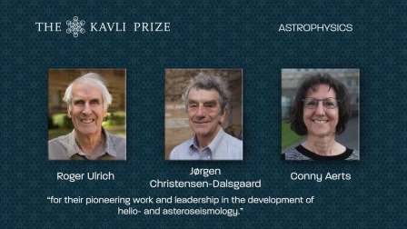
Jørgen Christensen-Dalsgaard, long-time Editor of Living Reviews in Solar Physics shares Kavli Prize in astrophysics
Sami Solanki, Editor-in-Chief of Living Reviews in Solar Physics, is awarded the 2022 George Ellery Hale Prize